8 Statistics
8.1 Introduction
In the Statistics course later in this degree program, you will have the opportunity to learn much more about statistics. In this chapter, I will give you a brief and gentle introduction to the foundational statistical concepts that you will likely encounter in the domain of IWO Psychology. That way, by the time you take the Statistics course, you will already be at least somewhat familiar with the foundational concepts, so it won’t be your first time learning the foundational concepts in that course. Repetition is great if we want to learn!
8.1.1 A special note from me to you
The field of Statistics is part of math, and many people have math-anxiety—they worry about not having skills to perform math-related tasks. I believe this is partially because of cultural norms about how math is taught in schools. Either way, I sincerely want to encourage you to not be discouraged when you’re learning about Statistics—or even Math in general!
When I was a student, I struggled with many concepts in Math and Statistics. If you use repeated recall (e.g., by using the Anki software) to memorize the foundational concepts of the field of Statistics, and you practice using those concepts in your everyday work, I promise you will feel more and more comfortable with statistical methods.
Be patient with yourself, and allow yourself to be exactly who you are…a person who is learning something new.
Also, don’t worry about memorizing all of the concepts in this chapter. I mostly want you to get the gist. I promise I won’t quiz you on all of the details.
8.2 Visually representing your data
When you collect data (whether it is sample data or an entire population’s data), you have a set of data, also known as a data set or dataset. You typically have data about several sample elements (or population elements, if your data are about an entire population). Almost always, you would store your data in a digital file that resembles a spreadsheet (also known as a table) with rows and columns. In that data file, each sample element (or population element) would be a row, and each variable would be a column. Table 8.1 illustrates a typical layout for a data file.
| Name | Salary | Job Satisfaction | Performance |
|---|---|---|---|
| Alex | 70,000 | 6 | 5 |
| Billie | 72,000 | 7 | 4 |
| Casey | 68,000 | 8 | 7 |
| Dani | 78,000 | 5 | 8 |
Visual representations of data are very useful, because most people find them easy to understand. In any domain of data-analysis, visual representations are commonly used to display a frequency distribution (typically using histograms, dot-histograms, and bar charts), and also to display the shape of the relationship between two variables (typically via a scatterplot, discussed further below).
A frequency distribution (also known simply as a distribution) tells how many times each type of datum occurs in whichever collection you’re looking at (e.g., in your dataset, or in a hypothetical population). You can represent a frequency distribution using a table, or you can make it into a chart like Figure 8.1, Figure 8.2, and Figure 8.4. You can make a frequency distribution for your data, regardless of whether your data are on a categorical or ordinal scale of measurement (e.g., Figure 8.4) or on an interval or ratio scale of measurement (e.g., Figure 8.1, Figure 8.2, Figure 8.3).
For a review of the four scales of measurement, see Table 7.1.
Bar charts can be used to summarize data in other ways, instead of only showing the frequencies. For example, Figure 8.5 is a bar chart showing the average (median) salaries of employees at ABC Company, categorized by their highest attained educational degree. Anytime you can put your data into separate categories, you can use a bar chart to summarize those data.
Another useful visual diagram is called a scatterplot, which I explain together with the concept of correlation in Section 8.7. Before we get there, let’s first make sure we understand the concepts of central tendency and variability in a frequency distribution, which I describe next.
8.3 Central tendency among data
When you have data from a variable and you want to figure out what is the most typical datum in your dataset for that variable, then a good answer to that is the central tendency of that data (i.e., the central tendency of the distribution of your data). There are several measures of central tendency. The three most popular measures of central tendency are: mean, median, and mode.
The two most popular uses for measuring central tendency on a variable X are:
- To know the “average” datum for a variable
Xin your dataset; - To compare two or more groups in terms of their respective central tendencies on a variable
X(e.g., compare the central tendency of Group A versus that of Group B).
8.3.1 Mean
The mean is the most popular measure of central tendency that researchers like to calculate.
If a dimension’s data are quantitative, then you can calculate the mean of that data. The mean (also known as the arithmetic average, or arithmetic mean) is the sum of the numeric data from that dimension across all the elements in your dataset, divided by how many elements you have.
If your dataset contains data for a quantitative dimensional variable X on your entire target population, then you can calculate the population mean of X (typically denoted via ). If your dataset only contains a sample from your target population, then you can calculate an estimate of the population mean for that variable
X—also known as the sample mean of X—(typically denoted via or
).
is the lowercase Greek letter mu (pronounced in English like “mew” or “moo”).
is read aloud as “the population mean of
X” or “the mean of X” or “mu X”.
is read aloud as “the sample mean of
X” or “the estimate of the population mean of X” or “the estimate of mu X” or “mu hat X”. is identical to
and is read aloud as “the sample mean of
X” or “the estimate of the population mean of X” or “X bar”. and
refer to the same thing.
The population mean of X is calculated with this formula:
Equation 8.1 is simply an algebraic expression to say: take the sum of all the data of the quantitative dimensional variable X, starting from the first element (i.e., ) in your population and ending with the final element (i.e.,
), and then divide by how many elements (
) you have in your population.
Equation 8.1 is often shortened to this more compact expression:
Equation 8.2 is simply another algebraic expression to say: take the sum of all the data of the quantitative dimensional variable X, starting from the first element in your population (indexed via ) and ending with the final element (indexed via
), and then divide by how many elements (
) you have in your population.
If your dataset only contains a sample from your target population, then the sample mean of X —also known as the estimate of the population mean of X—is calculated with this formula:
Notice Equation 8.2 and Equation 8.3 are fundamentally identical to each other—the only difference is in whether you’re using an entire population’s elements, or a sample’s
elements. However, for other types of population parameters and sample statistics, their formulas generally aren’t identical to each other.
8.3.2 Median
If you have data for a dimensional variable, and you put those data into a sequential order of increasing or decreasing amount of the essence of the variable, then the middle datum in that sequence is called the median of that data.
There is a formula to calculate the median of a variable, but that is beyond the scope of this course. Depending on whether your dataset contains your entire target population or only a sample, you can either calculate your target population’s median on a variable X, or instead you can calculate an estimate of the population’s median of X (also known as the sample median of X).
Among scholars, the median is increasing in popularity as a measure of central tendency (because of some advantages in statistical methods), but the mean is still more popular because most of the classic methods used in the field of statistics are based on calculations involving a mean.
TipFor example…
If employee salary is your dimensional variable, and we could put the employee salary data into sequential order of increasing (or decreasing) salary, like this:
$51k, $60k, $63k, $65k, $78k
The median of that data is the middle datum, which is $63k. If you have an even number of elements, then you would typically calculate the arithmetic average of the two middle elements and declare that average as your median.
8.3.3 Mode
The mode of a variable X is simply the most frequent datum of X in your dataset. The mode is not a very popular measure of central tendency, but it is useful because it can be used regardless of whether your variable is a dimension or not. In contrast, the mean and median can only work on dimensions.
TipFor example…
If job satisfaction is your variable measured on a scale from 1 through 5, with these data in your dataset: 1, 2, 3, 3, 4, 4, 4, 4, 4, 5, 5, then the mode is 4.
8.4 Variability among data
For the data from any variable X, a measure of the variability of that data refers to how much variety there is in that data.
Technically, there are several measures of variability that can be applied to data on a categorical or ordinal scale of measurement. However, those are beyond the scope of this course. Instead, we will focus on measures of variability for data on an interval or ratio scale of measurement.
For a review of the four scales of measurement, see Table 7.1.
Perhaps the simplest measure of variability is called range, which is simply the difference between the biggest numeric datum minus the smallest numeric datum.
TipFor example…
If job satisfaction is your variable measured on a scale from 1 through 5, with these data in your dataset: 1, 2, 3, 3, 4, 4, 4, 4, 4, 5, 5, then the range is calculated as the numeric difference between the biggest datum (i.e., 5) minus the smallest datum (i.e., 1), thus the range is .
The two most popular measures of variability for any variable X (if X is on an interval or ratio scale of measurement) are called the variance of X and the standard deviation of X.
The variance of X in an entire population—also known as the population variance of X—is typically denoted via . The variance of
X in a sample—also known as the sample variance of X—is typically denoted via or
.
is the lowercase Greek letter sigma.
is read aloud as “the population variance of
X” or “the variance of X” or “sigma squared X”.
is read aloud as “the sample variance of
X” or “the estimate of the population variance of X” or “the estimate of sigma X” or “sigma hat X”. and
refer to the same thing.
is read aloud as “the population’s standard deviation of
X” or “the standard deviation of X” or “sigma X”. is read aloud as “the sample’s standard deviation of
X” or “the estimate of the population’s standard deviation of X” or “sigma hat X”. and
refer to the same thing.
The standard deviation of X in an entire population—also known as the population’s standard deviation of X—is typically denoted via . The standard deviation of
X in a sample—also known as the sample standard deviation of X or the estimate of the population’s standard deviation of X—is typically denoted via or
.
As you can see from the notation, the standard deviation is simply the square root of the variance (i.e., ). Conversely, the variance is simply the standard deviation squared (i.e.,
). The standard deviation of
X has the same unit of measure as X (e.g., if X is measured in inches, then will also be in inches), but the variance of
X is measured in squared units of whatever X is measured in (e.g., if X is measured in inches, then will be in inches-squared, i.e., in2)
TipFor example…
If you have a sample of data on the variable job satisfaction, measured on a scale from 1 to 10, then the standard deviation of X (i.e., ) is also on a scale from 1 to 10, but the variance of
X (i.e., ) is on a scale from 12 to 102 (i.e., squared units of
job satisfaction). Thus, it’s easier to interpret the standard deviation, rather than the variance, and that is why scholars often prefer to report the standard deviations.
Figure 8.6 shows a dot-histogram of a frequency distribution with small variance, whereas Figure 8.7 has large variance. In the HTML version of this chapter (e.g., if you’re reading this in a web browser), Figure 8.6 and Figure 8.7 are interactive, such that you can change the variance of the variable X and see how the shape of its frequency distribution changes accordingly. As you can see, as the variance (or standard deviation) of X increases, the data are more spread out away from the mean of X. Conversely, as the variance (or standard deviation) decreases, the data are more concentrated toward the mean of X.
Although you don’t necessarily have to memorize the formulas for calculating a population or sample variance or standard deviation of a variable X, here they are if you’re curious:
8.5 Other aspects of the shape of a frequency distribution
Remember, at the beginning of this chapter I said a frequency distribution shows how many times each type of datum occurs (e.g., in your dataset, or in a hypothetical population). Figure 8.1, Figure 8.2, Figure 8.3, and Figure 8.4 are each a visual representation of a frequency distribution.
As you can see from those figures, visual representations of frequency distributions can be described in terms of their shape. When we describe their shape, we can describe the location of their central tendency (e.g., mean or median) and we can describe the amount of variability in the data (e.g., large versus small standard deviation).
In addition to central tendency and variability, there are two other aspects that are commonly used to describe a frequency distribution: skew and kurtosis.
The skew of a distribution describes how asymmetric (or symmetric) the distribution is. When the skew = 0, the distribution is perfectly symmetric. Figure 8.8 is interactive, and you can see how the shape of the distribution of X changes when you make the skew positive or negative.
There is a mathematical formula for the skew of a continuous variable, but that is beyond the scope of this course. For now, I can at least tell you a skew is typically denoted via the Greek lowercase letter gamma with a subscript 1 .
The kurtosis of a distribution describes how much the distribution looks pinched versus flat around its central tendency.
- If the central tendency looks relatively pinched (like a steep hill), then we say the distribution has positive excess kurtosis (we can also say the distribution is leptokurtic).
- If the central tendency has a relatively flat top, we say the distribution has negative excess kurtosis (we can also say the distribution is platykurtic).
Figure 8.9 is interactive, and you can see how the shape of the distribution of X changes when you change its kurtosis.
There is a mathematical formula for the kurtosis of a continuous variable, but that is beyond the scope of this course. For now, I can at least tell you a kurtosis is typically denoted via the Greek lowercase letter kappa or the Greek lowercase letter gamma with a subscript 2
.
I once had a professor who gave me this mnemonic: a leptokurtic distribution looks like a cliff you could leap off of (and land safely in the warm waters below), whereas a platykurtic distribution has tails that look like the bill of a duck-billed platypus.
8.6 The standard Normal distribution
The orange curvy line in Figure 8.10 shows the shape of a distribution that has its mean = 0, its standard deviation = 1, its skew = 0 (i.e., it is perfectly symmetric), and its kurtosis = 3. It resembles a bell (almost like an upside-down letter U). Because that distribution is so commonly used in statistics, it is given a special name: the standard Normal distribution (also known as the standard Gaussian distribution).
The dots in Figure 8.10 form a dot-histogram of a randomly-collected sample dataset (each datum is a dot) for a variable Z, from a population that has a Normal distribution for Z.
You can have other distributions that look bell-shaped, thus we would say they look like the Normal distribution, but they might not have the exact parameters of the standard Normal distribution.
8.7 Scatterplots and correlations
Scatterplots are visual charts that display the relationship among data from two quantitative dimensional variables, such that each sample (or population) element is represented by a dot on the chart.
Scatterplots can be a great visual way to show patterns in your data, such as a correlation. In Section 6.5.2 I briefly introduced the concept of a correlation, and then in Section 7.1.2 I briefly introduced the concept of a correlation coefficient. Here, I’ll give a bit more detail.
Imagine you have a dataset with information about individual workers, and for each element in your dataset (i.e., each person in your dataset) you have a measurement about two variables: job satisfaction and years at the job. Intuitively, the correlation coefficient of two variables (measured on one set of population or sample elements) is a number that tells us how closely the data from those two variables run together in a straight line if we plot our data from those two variables onto a scatterplot. If you’re reading the HTML version of this (e.g., in a web browser), you can get a good sense of what a correlation is if you adjust the slider in Figure 8.11 and see how the shape of the X Y scatterplot changes as you change the correlation coefficient.
Keep in mind: in this scatterplot each dot is one person.
Thus, a correlation is a rectilinear pattern among the data from two quantitative dimensional variables, such that the data from one variable tend to go in one direction (i.e., higher, or lower) as the data from the other variable (on the same sample elements or population elements) go in one direction for the same elements. For example, Figure 8.12 is a scatterplot showing a positive correlation (meaning: the data of the two variables tend to go in the same direction), whereas Figure 8.13 is a scatterplot with a negative correlation (meaning: the data from the two variables tend to go in opposite directions).
The word rectilinear means “straight line”. The word curvilinear means “curvy line”. The word linear means “of or relating to a line”, but you would need to clarify what type of line is being referring to. For better or worse, many scholars simply use the word linear when they really mean rectilinear.
Job Satisfaction (1–10) versus Years at the job (0–45) at ABC Company. The two variables have a positive correlation: job satisfaction tends to be higher among employees who’ve been at ABC Company longer. In other words, the two variables tend to go in the same direction. An orange line visually emphasizes the correlation trend.
Keep in mind: in this scatterplot each dot is one person.
Count of ethical violations versus Conscientiousness (1–10) at ABC Company. The two variables have a negative correlation: the number of ethical violations tends to be lower as the employee’s conscientiousness is higher. In other words, the two variables tend to go in opposite directions.
Keep in mind: in this scatterplot each dot is one person.
When you have two variables (e.g., X and Y) that are each on an interval or ratio scale of measurement, you can calculate the Pearson correlation coefficient for those two variables—although most people tend to simply call it the correlation coefficient or the correlation. After calculating it, we could say “we’ve calculated the correlation of X and Y”.
There are other types of correlation coefficients besides Pearson’s, such as Spearman’s correlation and Kendall’s correlation. Those are beyond the scope of this course. A more formal name for the Pearson correlation coefficient is the Pearson product-moment correlation coefficient.
A population’s correlation coefficient (sometimes simply called a population correlation) is typically denoted via , which is the Greek lowercase letter rho. The sample correlation coefficient (also known as the sample estimate of the population’s correlation coefficient) is typically denoted via either
or the English lowercase letter
.
The Greek lowercase letter rho () is pronounced /roʊ/, like “row your boat”.
is read aloud as “rho hat” or “the estimate of rho”. Although
looks like a curvy English letter p, you can usually figure out it is the lowercase letter rho if the context is talking about a population’s correlation coefficient.
A correlation coefficient is always somewhere between and
(i.e.,
, and
). For example, you might see
, or
. When
, there is no correlation at all among those two variables in the sample data. When
or
, there is a perfect correlation among those two variables. In Psychology—including IWO Psychology—we almost never see
nor
in any sample dataset. In Figure 8.11, if you move the slider to the left of the middle, the correlation is negative and you can see the scatterplot looks like it’s trending downward (if you imagine you’re “reading” the scatterplot from left to right). If you move the slider to the right of the middle, the correlation becomes positive and you can see the scatterplot looks like it’s trending upward (again, if you imagine you’re “reading” the scatterplot from left to right)
Although you don’t need to memorize it for this course, in case you’re curious here are formulas to calculate and
(also typically written as
):
As you can imagine, correlation is a very popular concept, because it’s a simple and straightforward summary of the rectilinear relationship between the data about two variables measured from one set of elements.
8.8 Descriptive statistics vs. Inferential statistics
Recall from Section 7.2:
- a population is any set we want to understand;
- a sample is any subset of a population;
- a parameter is any numeric characteristic that describes a population;
- a statistic is any numeric characteristic that describes a sample.
Whenever we can’t access an entire population we’re interested in understanding, we can use a sample from that population to help us make inferences about our target population. Often, we calculate numeric summaries of our sample data to try to estimate population parameters. Table 7.3 from Section 7.2 provides examples of sample statistics and their corresponding population parameters.
TipFor example…
I could apply a mathematical formula onto the salary data of employees in my sample, to estimate the average salary of my target population. Of course, the validity of that method depends on several assumptions (e.g., is my sample representative of my target population?).
When you use your sample statistics to describe or summarize your sample data, without focusing on describing your inference about a target population, we would say you are providing descriptive statistics (that’s how scientists—including IWO Psychologists—and statisticians use that term).
When you use your sample statistics to describe or summarize your inference about a target population, we would say you are providing inferential statistics (again, that’s how scientists—including IWO Psychologists—and statisticians use that term).
However, many scholars colloquially use the phrase “descriptive statistics” anytime they are referring to simple numeric summaries (e.g., mean, median, standard deviation, etc.), regardless of whether or not they are estimating the population versions of those numbers.
TipFor example…
You could calculate the variance of the salaries of workers in your sample data, without trying to infer the population’s variance of salaries. That would be a descriptive statistic.
Alternatively, you could use your sample data of salaries to calculate an estimate of the population’s variance of salaries. That would be an inferential statistic.
In the next sections of this chapter, I explain two of the most common methods for using inferential statistics:
- parameter estimation with confidence intervals;
- null-hypothesis significance testing (NHST).
8.9 An important ingredient for inferential statistics: a Sampling Distribution
Remember, inferential statistics attempt to use sample data to describe an entire target population. To do that, we rely on something called a sampling distribution. Perhaps an example is the best way to explain what a sampling distribution is. Imagine you collect a random sample of 100 workers in the USA and they each tell you their annual salary, and you calculate your sample mean annual salary and write it down. Then, you start over with a new random sample of 100 workers and write down their mean annual salary. You keep doing that with new random samples, and you do it a million times. Now, you have a million sample means of annual salary (i.e., each sample mean belongs to one of your million samples of 100 workers) and you can make a frequency distribution of those sample means. Thus, you have a frequency distribution where each datum is not an individual person, but rather each datum is a sample mean from one of your million samples of 100 workers. That frequency distribution is a sampling distribution of the mean annual salary!
A sampling distribution is a theoretical distribution of all the possible the numeric values of a sample statistic if you imagine being able to collect all possible samples (each being the same size) from your target population. Fortunately, statisticians have figured out mathematical formulas to produce a sampling distribution for any typical statistic, so you don’t actually have to collect millions of separate samples.
In science—including IWO Psychology—when we’re dealing with sampling distributions, we often focus on a sampling distribution of a mean of a variable (e.g., for a variable X, we’re often interested in the sampling distribution of , i.e., the sampling distribution of the mean of
X). There are two very important properties about the sampling distribution of a mean:
- When you use an unbiased sampling method (e.g., random sampling) to obtain your samples from your target population, then the mean of the sampling distribution of the mean of
Xis equal to the target population’s mean ofX. - When you use an unbiased sampling method (e.g., random sampling) to obtain your samples from your target population, then the sampling distribution of the mean of
Xhas the shape of the Normal distribution if the sample isn’t tiny. This is because of an interesting mathematical truth known as the Central Limit Theorem (which is beyond the scope of this course).
The top of Figure 8.14 shows a line diagram representing the sampling distribution of the mean of a variable. At the center is the mean () of the entire sampling distribution. Assuming we used an unbiased sampling method (e.g., random sampling) to obtain each sample, then the mean of the sampling distribution is equal to the population’s mean.
Just like you can calculate the standard deviation of a frequency distribution, you can do the same for a sampling distribution—the only difference is we call it the standard error (instead of the standard deviation) of the sampling distribution. So, the standard error of a sampling distribution is simply the standard deviation of the sampling distribution.
Note
When the standard error of our sampling distribution is large, we can expect a lot of variation (i.e., a lot of disagreement) in the results from one sample to another (e.g., one sample’s mean might be $50K whereas another sample’s mean might be $90K). When the standard error is small, we can expect little variation (i.e., more agreement) in the results from one sample to another (e.g., one sample’s mean might be $50K whereas another sample’s might be $51K).
8.10 Estimating a population parameter by using a confidence interval
When we use a sample statistic to try to arrive at a parameter estimate (i.e., an estimate of the parameter that corresponds to our sample statistic), we can use either a point estimate or instead we can use an interval estimate (also known as a confidence interval). A point estimate is a single number that is calculated from the sample data (using a statistical formula), and that single number is declared our parameter estimate (i.e., our estimate of the population parameter).
A better approach is to take that point estimate and surround it with a range of numbers that are also good candidates for the parameter estimate. That range is called an interval estimate or a confidence interval. The confidence interval (also abbreviated as CI) of our target population parameter is a range of numbers that has a specified probability of containing the true population parameter (e.g., the population mean, or the population correlation coefficient, or the population regression coefficient). In science, we almost always use our actual sample dataset to calculate a 95% confidence interval (also written as 95% CI). The 95% CI has a 95% probability of containing the true population parameter. Using special mathematical formulas (which are beyond the scope of this course), we typically use a sampling distribution (of whichever parameter we’re interested in) to help us calculate the 95% CI.
A 95% confidence interval is commonly used in science, because it feels like a good “sweet spot”. If we increase the confidence level to something like 99%, then the interval would get much larger (e.g., there’s a 99.999% chance that the average annual salary of workers in the USA is between $0 and $1 million), thus it would be less useful. If we decreased the confidence level to something like 50%, then the interval would shrink but we wouldn’t have much confidence that it contains the true population parameter.
TipFor example…
For example, let’s imagine our variable is the annual salary of workers, and the true population mean of annual salary is $60K. Imagine we randomly obtain a sample of 100 workers, and we calculate the 95% CI for the mean of annual salary from that sample is (that’s the typical way of writing “the range is from $44K to $77K”). Then we randomly obtain another sample of 100 workers and calculate the 95% CI for the mean of
annual salary from that sample is . We keep collecting new random samples of 100 workers many times until we end up with a collection of a million samples, each one with its own 95% CI for the mean of
annual salary. For 95% of those million samples, each of their 95% CIs will contain the true population mean of $60K. For the remaining 5% of those million samples, none of their 95% CIs will contain the true population mean of $60K.
As an illustrative example, consider Figure 8.14 which focuses on a 50% CI instead of a 95% CI. The bottom of Figure 8.14 shows 20 randomly-collected samples, and each sample contains 10 elements indicated via black dots. The dashed vertical line shows the location of the population mean along the horizontal number-line. Each dot to the right of the dashed vertical line represents a datum that is bigger than the population mean, and each dot to the left of the dashed vertical line represents a datum that is smaller than the population mean. For each sample, the 50% CI of that sample is shown as a red or blue line, and the sample mean of each sample is shown as a diamond. The blue confidence intervals overlap with the true population mean, whereas the red confidence intervals don’t. Indeed, there are 10 blue confidence intervals, and 10 red ones. That is because each of those confidence intervals is a 50% CI, thus, by definition, each of those CIs has a 50% chance of containing the true population parameter. If we would’ve calculated a 95% CI instead, then each CI would’ve been wider (i.e., a bigger range), and 19 of them would’ve been blue (that’s 95% of 20 samples) and only one of them would’ve been red (that’s 5% of 20 samples).
In Figure 8.14, each sample’s confidence interval is calculated using the same mathematical formula. The only reason why each sample has a slightly different confidence interval is because each sample contains slightly different data, as you can see from the location of the black dots in each sample.
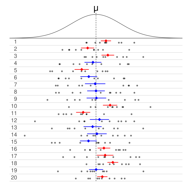

What we hope to achieve is a confidence interval that is narrow (i.e., a small range of numbers, not a wide range) while still giving us a high degree of confidence that it contains the true population parameter. The width (or narrowness) of a confidence interval depends on how much confidence you want to have, and how big your sample size is (i.e., the number of elements in our sample). If we want to stick to a 95% CI, then we can try to narrow the width of the 95% CI by increasing our sample size. In other words, a 95% CI calculated from a sample of 500 elements will be narrower (i.e., better) than a 95% CI calculated from a sample of 100 elements.
8.11 A classic approach for inferential statistics: Null-Hypothesis Significance Testing (NHST)
Null-Hypothesis Significance Testing (NHST; also known simply as hypothesis testing, though that wording is more vague) is the name of a classic method for making an inference about a population, by using an inferential statistic. You can think of the method like a sequence of steps in a food recipe.
Remember in Section 7.2.3 I said the field of statistics is currently somewhat bifurcated into two separate approaches: frequentist statistics and Bayesian statistics. Frequentist statistics is classic, and most students are taught frequentist statistics by default. NHST is part of the world of frequentist statistics, and it is very common among scientists—including IWO Psychologists. Although there are similar techniques in Bayesian statistics, they are currently beyond the scope of a typical introductory research methods course. Thus, I focus on NHST in this chapter.
8.11.1 Step 1/4: create a null hypothesis and an alternative hypothesis…
The first step in NHST is: you must write a null hypothesis and an alternative hypothesis. The alternative hypothesis (typically denoted via the symbol ) is the hypothesis that you believe is true about your target population (e.g., a hypothesis that you created from a theory). The null hypothesis (typically denoted via the symbol
) says your alternative hypothesis is not true, and more specifically we almost always make our null hypothesis say something like: “in the population, there is no pattern among the data about the concepts in the hypothesis”. Examples of typical null hypotheses and alternative hypotheses are listed in Table 8.2. Whenever you write a hypothesis, it must involve at least one variable (e.g., in Table 8.2 the variables are written in
code font), therefore your hypotheses are falsifiable statements (e.g., guesses) about one or more population parameters that correspond to the variable(s) in your hypotheses.
NHST is simply a method to help us figure out whether our sample data support the null hypothesis (about our target population) or the alternative hypothesis (about our target population).
| Null hypotheses |
Alternative hypothesis |
|---|---|
At ABC Company, the average salary of men is no different than that of women. |
At ABC Company, the average salary of men is larger than that of women. |
At XYZ Company, the weekly average number of meetings in the marketing department, engineering department, and accounting department are no different than each other. |
At XYZ Company, the weekly average number of meetings in the marketing department, engineering department, and accounting department are different than each other. |
In the USA, the correlation between a person’s level of education and annual income is zero. |
In the USA, the correlation between a person’s level of education and annual income is positive. |
8.11.2 Step 2/4: choose an alpha level…
Next, before you analyze your sample dataset, you must choose something called an alpha level (also called a level of statistical significance or simply the level of significance; it is also written like this: level). The alpha level describes the level at which we would conclude that our sample statistic (e.g., a sample mean, or a sample correlation coefficient, or a sample regression coefficient, etc.) would be very rare if we temporarily imagine the null hypothesis is true. The reason why we need an alpha level is because there’s always some unlucky chance that the sample we collect will contain rare data that doesn’t really match the target population overall. If we get an unluckily rare sample, we wouldn’t want to infer the population is similar to our sample. However, we almost never know with 100% certainty what the true population parameters are, thus we can’t know for certain whether our sample is rare. Thus, in NHST, we temporarily imagine the null hypothesis is true, and then we can figure out how rare our actual sample statistic would be in that imaginary world. Thus, our chosen alpha level establishes a numeric threshold (expressed as a percent) that defines the point at which we will decide that it would’ve been too rare to get the sample statistic we got from our actual sample, if we temporarily imagine the null hypothesis is actually true.
In the vast majority of situations in the social and/or behavioral sciences—including IWO Psychology—we typically choose an alpha level of 5%, which is also written as (because the decimal number 0.05 is another way of writing 5%).
There’s a good reason why we typically choose an alpha level of 0.05. I explain in Section 8.11.5.
Many scholars misunderstand the meaning of the alpha level. The example in this next For example… block should help clarify it:
TipFor example…
Imagine our actual hypothesis (i.e., the alternative hypothesis) is that the population correlation between a person’s age and annual income is positive in the USA (i.e., ), and our null hypothesis is that the population correlation is zero (i.e.,
). Let’s say we want our alpha level to be 5% (also written as
). Then, let’s say we calculate the sample correlation (
) between
age and annual income in our sample and we see it is .
On the surface, obviously doesn’t equal
, but in NHST we want to know whether
is statistically significantly different than
. Indeed, if our sample size is very small, it is very possible that
will not be statistically significantly different than
. If
is statistically significantly different than
, then we will reject the null hypothesis. If
is not statistically significantly different than
, then we will not reject the null hypothesis.
To figure out whether is statistically significantly different than
, we temporarily imagine the null hypothesis is true (i.e.,
), and we use a mathematical formula (beyond the scope of this course) to establish a sampling distribution that corresponds to the population correlation (
) being zero (because that is what the null hypothesis says). Then, we use that sampling distribution to see how rare our actual sample correlation (
) would be in that imaginary world. The sampling distribution will tell us the percent of the time (i.e., the percent of all theoretically possible samples) that would’ve given us a sample correlation that is at least as big as
.
Because we chose our alpha level to be 5%, we essentially said our decision rule is this: if the sampling distribution says we would’ve obtained a sample correlation at least as big as in only 5% or fewer of all the possible samples in that imaginary world, then we reject the null hypothesis. Otherwise, if the sampling distribution says we would’ve obtained a sample correlation at least as big as
in more than 5% of all possible samples in that imaginary world, then we don’t reject the null hypothesis.
8.11.3 Step 3/4: obtain a p-value from a statistical test…
After you’ve chosen an alpha level (typically ), you can then conduct whichever statistical test matches your hypothesis (e.g., a
-test, an ANOVA, or perhaps a regression analysis). In this research methods course, we won’t focus on the mathematical details of any of those statistical tests (you will learn about them in the statistics course), but in the next section of this chapter I will give you a brief conceptual description of what each of those tests accomplishes and how you can decide which one is appropriate for your hypothesis.
Regardless of which statistical test you use, each of them will conclude by giving you something called a -value (which is shorthand for probability value) for your sample statistic. To understand what the
-value is, we need to go back to the sampling distribution from when we temporarily imagined the null hypothesis is true. Remember, for a statistic we’re interested in, the sampling distribution of that statistic is a distribution of all of the possible results for that statistic from all of the possible samples that could theoretically exist. In NHST, we temporarily imagine the null hypothesis is true and then we use mathematical formulas (beyond the scope of this course) to figure out what the theoretical sampling distribution would’ve been in that imaginary world. In that sampling distribution, some of its samples would’ve given us the same sample statistic that we actually got from our actual sample dataset. Also, some of those samples would’ve given us a sample statistic even more extreme than our actual sample statistic (e.g., a mean that is bigger, or a correlation that is bigger, or a regression coefficient that is bigger). There might be only a few of those extreme samples from the entire sampling distribution, or there might be many of them. Either way, by using the sampling distribution, we can know the answer to this question: what percentage of the samples from the hypothetical sampling distribution would’ve given us a sample statistic that is at least as extreme as our actual sample statistic? That percentage is the
-value for our actual sample statistic.
Many scholars (even those with PhDs!) incorrectly believe the -value tells you the probability that your sample statistic matches the population parameter, or even the probability that the null hypothesis is true. Be very careful before you believe what anyone says about statistical methods, even if they have a PhD! When in doubt, get your knowledge from a book about statistical methods, written by a statistician.
8.11.4 Step 4/4: compare your p-value versus your alpha level, to make a decision about whether to reject the null hypothesis…
After we calculate the -value for our sample statistic, we then compare the
-value versus our chosen alpha level:
- If the
-value is less than or equal to our chosen alpha level, we say our sample statistic is statistically significant at our chosen alpha level, and we reject the null hypothesis (and therefore we tentatively support the alternative hypothesis).
- For example: “the sample correlation was statistically significant at the 0.05 alpha level,
.”
- For example: “the sample correlation was statistically significant at the 0.05 alpha level,
- If the
- For example: “the sample correlation was not statistically significant at the 0.05 alpha level,
.”
- For example: “the sample correlation was not statistically significant at the 0.05 alpha level,
This rhyme might help you: “if the is low, reject the null!”
Thus, a sample statistic is statistically significant at our chosen alpha level if the -value of that sample statistic is less than or equal to our chosen alpha level.
This next For example… block is a continuation of the previous example, and it illustrates how we use the -value to make a decision to reject the null hypothesis:
TipFor example…
Let’s go back to the example from the prior For example… block about the population correlation between a person’s age and annual income in the USA. Remember, we chose an alpha level of 5% (i.e., ).
In that scenario, we needed to figure out whether our actual sample correlation () is statistically significantly different than
. To do that, we would conduct a
-test to compare
from our sample versus the null hypothesis’ claim that
. Let’s imagine we calculate the results of our
-test and it says the
-value for our sample correlation (
) is 0.077 (that’s another way of writing 7.7%).
In other words, when the -value is 0.077, it tells us this: in the imaginary world where we assume the null hypothesis is true (i.e., that
), we would’ve had a 7.7% chance of ending up with a sample correlation at least as big as the one we got in our actual sample (
). In more technical terms, it’s saying only 7.7% of all the samples from the hypothetical sampling distribution (if the null hypothesis were true) would’ve given us a sample correlation at least as big as
.
Thus, because our chosen alpha level was (i.e., 5%) and we ended up with a
-value of
(i.e., 7.7%), our sample statistic is less rare than the 5% alpha level we chose. Thus, we say our sample correlation is not statistically significant at the 0.05 alpha level, and we don’t reject the null hypothesis.
As you can see, just because a sample statistic seems to be different than the null hypothesis on first glance, the sample statistic might not be statistically significantly different than the null hypothesis.
WarningStatistical Significance versus Practical Significance
Unfortunately, researchers use NHST so much that they often just say significant instead of saying statistically significant. For people who don’t understand NHST, they might read a headline that says: “New research shows the color purple is a significant predictor of performance” even though the actual analysis only showed that the color purple in an office had a correlation with performance that was statistically significantly different than zero at the chosen alpha level. If the sample size was very large, the correlation could’ve been very small () but still statistically significantly different than zero at the 0.05 alpha level if the correlation’s
-value is
. Those types of results happen all the time when you have large samples.
As you can see, just because a sample statistic is statistically significant doesn’t mean it is practically significant nor useful in reality. If the correlation between one’s performance and having the color purple in an office is , the correlation is so small that it’s practically telling us we can’t actually use the
color purple to predict someone’s performance.
8.11.5 The two types of errors in NHST: Type I versus Type II errors
In NHST, a Type I error (also called a false positive) occurs when you reject a null hypothesis that is actually true about your target population. A Type II error (also called a false negative) occurs when you don’t reject a null hypothesis that is actually false about your target population.
The Type I error rate is the probability of making a Type I error. The Type II error rate is the probability of making a Type II error.
The Type I error rate is the same as the alpha level. If your chosen alpha level is 5%, then you have a 5% probability of making a Type I error. If you want to lower your Type I error rate, you can choose a smaller alpha level. However, if you do that, you will automatically increase the Type II error rate. Conversely, if you raise the alpha level (therefore increasing the Type I error rate), you automatically lower the Type II error rate.
As I said before, in the vast majority of situations in the social and/or behavioral sciences—including IWO Psychology—we typically choose an alpha level of 5%, as a “sweet spot” that gives us a reasonably low Type I error rate, without a big Type II error rate. Of course, this is just a rule of thumb, and you can use whatever alpha level you believe is appropriate for your specific study (and hopefully you would provide a reasonable explanation for your choice).
A Type I error is called a false positive because it would lead us to essentially accept the alternative hypothesis (because we incorrectly decided to reject the null hypothesis). A Type II error is called a false negative because it would lead us to essentially reject the alternative hypothesis (because we incorrectly decided to not reject the null hypothesis). Thus, the word error in Type I error and Type II error refer to the status of our decision about the null hypothesis, but the words positive and negative in false positive and false negative refer to the status of our decision’s impact on the alternative hypothesis.
8.12 The most common inferential statistical procedures in NHST: t-test, F-test, ANOVA, regression…they’re all simply types of the general linear model
Traditionally (and still today in many graduate statistics courses), students are taught several inferential statistical procedures such as the -test, and several versions of the analysis of variance (ANOVA, ANCOVA, MANOVA, MANCOVA),
-test, and regression. All of those are options you can use in NHST. However, few courses focus on showing how all of those procedures are simply types of a general system known as the general linear model. That type of knowledge greatly simplifies what would otherwise be a long list of seemingly separate procedures, each for a slightly different scenario. Fortunately for you, the statistics course in this degree program does exactly that.
Indeed, it is a bit of a shame that more statistics courses don’t teach modern statistical methods from the perspective of the general linear model, especially because statisticians figured it out by the 1960s.
Still, for the sake of being able to understand the vast majority of published research in arguably every domain of science—including IWO Psychology—it is worth knowing the general purpose of the aforementioned classic types of statistical procedures and their classic names, which I provide below.
8.12.1 t-test
A -test is a classic name for an inferential statistical procedure that is commonly used in NHST when we want to test this null hypothesis: “the population parameter we’re interested in is zero”. The parameter we’re interested in is typically a mean, or a correlation, or a regression coefficient. If the result leads us to reject the null hypothesis, we tentatively accept that the sample statistic is statistically significantly different than zero.
The -test is most commonly used for these scenarios:
- Figuring out whether the mean of
Xin one group of people is statistically significantly different than the mean ofXin another group of people. - Figuring out whether the mean of
Xin a group of people at timepoint 1 is statistically significantly different than the mean ofXin the same group of people at timepoint 2. - Figuring out whether the correlation between
XandYis statistically significantly different than zero. - Figuring out whether the regression coefficient of a predictor variable
Xon an outcome variableYis statistically significantly different than zero.
8.12.2 F-test, ANOVA, and regression
An -test is a classic name for an inferential statistical procedure that is commonly used in NHST. A good definition of an
-test is beyond the scope of this course. However, the important thing to know for now is that the
-test is commonly used in NHST when you want to conduct an ANOVA or a regression analysis.
For now, I can at least tell you this optional bit of information which you don’t need to remember for this course: an -test is any hypothesis test whose test statistic has an
distribution under the null hypothesis.
One version of the -test is used when we conduct an ANOVA (analysis of variance). ANOVA is a classic name for an inferential statistical procedure that is commonly used in NHST when we want to test this null hypothesis: “the population means of
X in each of three or more groups are all equal to each other”. If the result leads us to reject the null hypothesis, we tentatively accept that the mean of X in at least one of the groups is statistically significantly different than the rest.
ANCOVA, MANOVA, and MANCOVA are merely slightly more complicated versions of ANOVA, but they are beyond the scope of this course (and you will learn about them in the statistics course in this degree program).
Another version of the -test is used in a regression analysis. A regression analysis is any of a family of inferential statistical methods in which we want to see how the datum of an outcome variable
Y (which is on an interval or ratio scale of measurement) changes as the data of one or more predictor variables X₁, X₂, …, Xₙ changes.
Often you will hear people describe regression analysis as “a way to predict an outcome variable Y, based on one or more predictor variables X₁, X₂, …, Xₙ”. What they mean by that is: if we know how the datum of Y changes as the data of the predictor variables change, then we can use that knowledge to predict what the datum of Y should be if we know what the data of the predictor variables are.
When we use an -test in a regression analysis, we test this null hypothesis: all of the population regression coefficients in our regression model are equal to zero. If the result leads us to reject the null hypothesis, we tentatively accept that at least one of the regression coefficients in our regression model is statistically significantly different than zero.
As I mentioned earlier in the section about -tests, we also typically use t-tests when we’re conducting a regression analysis. In that scenario, we use the
-test to test this null hypothesis: “this specific regression coefficient (
) is zero in the population”. If the result leads us to reject the null hypothesis, we tentatively accept that the particular regression coefficient (
) we tested is statistically significantly different than zero.
Scholars typically say any of these when they’re conducting a regression analysis: I’m estimating a regression model; I’m running a regression analysis; I’m running a regression model; I’m testing a regression model.
8.13 Suggested Readings
You will take a Statistics course in this degree program, but if you are eager to learn more about statistics before taking that course, here are some books I can personally recommend:
References
Shao, J. (2003). Mathematical Statistics (2nd edition). Springer.
Wackerly, D., Mendenhall, W., & Scheaffer, R. L. (2008). Mathematical Statistics with Applications (7th edition). Thomson Brooks/Cole.
Wasserman, L. (2003). All of Statistics: A Concise Course in Statistical Inference (First Edition). Springer.